Tip #46 - Excel AutoFit Column Width

100 Computer Tips in 100 Days

Tip #46 - Excel AutoFit Column Width

When you begin an Excel spreadsheet, all of the columns and rows start out the same default width and height. The default column width is 8.11 characters or 80 pixels. The default row height is about 14.4 characters or 24 pixels (it varies by version). As long as the information you put in the columns and rows fit in those constraints you are golden. Unfortunately the world isn't that organized and you will probably need to change the column and row sizes. That’s where Autofit comes in.

I recommend you input a row or two of information before you change the column width. This will give Excel some idea about the type of information you plan on putting in the columns and rows and enable you to use the AutoFit feature. The rows and columns will be resized to the widest/tallest entry in the column/row.

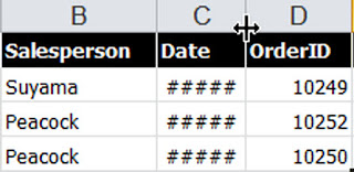
You can AutoFit one column or all of the columns depending on how many you select in the worksheet. To AutoFit one column, column C in the example (see screen shot) place your mouse on the vertical line that separates that column in the column heading from the column to the right,  and double click the mouse.  In the screen shot, column C would be adjusted.

If you needed to AutoFit all of the columns in the worksheet as you often need to when using imported data, you need to select the entire document. You can do this by using a keyboard method (Ctrl + a, Command + a for Apple users) or by clicking the select all box in the extreme upper left corner of the workbook, where the row numbers and the column letters intersect.  Once the worksheet is selected, move your mouse on the vertical line in the column header between any two columns and double click the mouse button.

Use the same strategies to resize the row height.

I have noticed that sometimes Excel resists the AutoFit double click. In those cases I select the entire document and manually drag the column width to make it very wide, much wider than the maximum size I need. I release the mouse button and then go back between any two columns and perform a double click. Magically Excel now knows that you mean business and reduces the columns to a best fit option. You might also have to double click the horizontal line between any of the rows to reduce the height of all of the rows.

My book, 100 Amazing Computer Tips - Shortcuts, Tricks, and Advice to Help Everyone from Novice to Professional, is available NOW at Amazon.com and Barnes & Noble in both print and ebook formats. There's also a handy link on top right side of this window.

Happy computing!

Diane

Don't forget to click the Subscribe to 100 Computer Tips in 100 Days via email link on the right side of the screen so you get email alerts when Diane adds a new post.