Named Cells and Ranger in Excel

Great Computer Tips

Named Cells and Ranges in Excel

Naming cells

Cells already have names such as A1, B27, etc. but you can also give them names to make it easier to reference that specific cell, making the cell address (name) an absolute reference rather than the default relative address. In the image below, you might want to name cells A1 through D10 but since you might be expanding your product list we'll give columns A through D a name.

• Start by selecting the single cell, range of cells, or columns you want to name.
• Click in the name box (the name box is in the upper left side of your screen, just above the first column, see image to the right) and type a name for your cells.
• Press the Enter/Return key. This step is very important.

If we called this area of our worksheet "table" we would be able to use the word "table" in our formula and Excel would know that we were referencing these cells on this worksheet. 

Note: When naming cells you need to remember that you can not use spaces and the name can not begin with a number. Also remember, the name must be unique in the workbook because the name refers to a location in a specific worksheet in the workbook. 

Using Names in Formulas

Once you have named a cell or range of cells, you can insert that name into your formula. The formula becomes easier to decipher and doesn't require adding $'s to the cell address to make it a fixed location. The formula could be =SUM(sales) rather than =SUM(A3:G27).

Viewing the Names in a Workbook

You can easily view all the names in the workbook by clicking the down arrow on the right side of the Name Box. The list is always viewed in alphabetical order.

Happy Computing!

Diane

Don't forget to click the Subscribe to 100 Computer Tips in 100 Days via email link on the right side of the screen so you get email alerts when Diane adds a new post.

Want more tech news or interesting links? You'll get plenty of both if you keep up with Diane McKeever, the writer of 100 Computer Tips in 100 Days, by subscribing to her Facebook posts or visiting her web page, www.dianemckeever.com

Excel - Converting Zip Codes to City and State

 100 Computer Tips in 100 Days

Excel - Converting Zip Codes to City and State


In my new position, I offer free webinars to people who want to improve their chances of business success. These folks sign up with their name, email, and zip code. I was curious about their location and was amazed that Excel could convert the zip codes into city and state locations. BTW, I believe this feature is only available in the 365 version of Excel.

To do this you need to start by converting the zip code column to text. 

1. Select the zip code column by clicking on the letter of the column
   
2. From the Home Tab, Number Group, choose Text

Select all the zip codes in the list 

1. Click the first zip code and use the Ctrl + down arrow key
2. From the Data Tab, Data Type Group, choose Geography

You will see a new icon to the left of the zip code entries

Select the first zip code in your list. You will see a new icon on the right, the Insert Data icon. Click it and choose "City". 

The City and State will be inserted into the cell to the right of the zip code. Use the fill handle to fill this code down the rest of your list. You may get some wonky entries if incorrect data is entered. 

I hope you enjoyed this tip. Please share the link to your friends.

Diane

Diane McKeever, CPP

Certified Patient Person

Don't forget to click the Subscribe to 100 Computer Tips in 100 Days via email link on the right side of the screen so you get email alerts when Diane adds a new post.

Excel's Amazing VLOOKUP Function

Great Computer Tips

Excel's Amazing LOOKUP Functions

The LOOKUP functions in Excel are so powerful but so confusing to many. Part of the problem is the terms that Excel uses when defining the arguments. Let's see if I can make things clear for you.

LOOKUP functions copy information from a table based on data in specified cells. You see LOOKUP functions in use all of the time. The bar code scanner in stores uses a form of lookup. The scanner identifies the UPC number and returns the name of the item and the price from a list stored on the server. The UPC is the trigger or the number being looked up and the price is in one column and the name of the item is stored in another column. I can hear you saying that you're not selling products and don't use UPC numbers. Another example of a lookup is auto-entering customer information using a customer number.

This VLOOKUP uses an Item # that is common to the worksheet and the Lookup Table to automatically import information.

For many years I was in charge of scoring sailboat races and we used an Excel worksheet to accomplish this. When a boat came out to race we entered the sail number and the spreadsheet looked up information from another sheet that had hundreds of sailboats listed. The sail number would trigger the lookup and the name of the boat would be automatically entered as well as the name of the skipper and the handicap.

In a recent tip for parsing date information into individual segments, I suggested the use of the WEEKDAY function to determine the day of the week that a particular day falls on. The result of this formula is a number from 1 to 7. If you wanted to convert those numbers to day names (Sun, Mon, etc.) then you would consider using a lookup to accomplish this task.

So now that you have some ideas about how you would use a lookup let's get started.

Setting up the Lookup table
The data in the table needs to be set up so that the lookup number (the information you are looking for such as the UPC code or model number) is in the leftmost column and is sorted in ascending order (from smallest to largest). To make it easier to identify the location of the table the next step would be to name the table area.

Naming cells
Cells already have names such as A1, B27, etc. but you can also give them names to make it easier to reference that specific cell, making the cell address (name) an absolute reference rather than the default relative address. In the image above you would want to name cells A1 through D10 but because you might be adding to your product list we'll give columns A through D a name.

• Start by selecting the cells or columns you want to name.
• Click in the name box (the name box is in the upper left side of your screen, just above the first column, see image to the right) and type a name for your cells.
• Press the Enter/Return key. This step is very important.

If we called this area of our worksheet "table" we would be able to use the word table in our formula and Excel would know that we were referencing these cells on this worksheet. Note: When naming cells you need to remember that you can not use spaces and the name can not begin with a number.

Inserting the LOOKUP Function

Now that we've got the data range named lets look at how to construct the VLOOKUP function. Look at the image below, we will be inserting information in the worksheet on the left by looking it up in the sheet on the right.

In the example we will create a function to look up the description of an item based on the Item #. In the first cell in the description field, choose VLOOKUP from the Formulas tab, Function Library group, Lookup & Reference option. We are using a VLOOKUP rather than a HLOOKUP because the data we're looking up from in the worksheet on the right  is structured in a vertical format.

• In the function builder dialog box put in the cell address of the trigger cell. In this case it is cell B20, the cell that will contain the item #. 
• In the second field type the name that you gave your look up information. I named mine "table" so that's what I typed in here. 
• In the third box identify the column in the worksheet on the right that has the information you want returned. The Code (Item #)  is column 1, Description is column 2, Price is column 3 and Color is column 4. In this case we would type a 2. 
• If it is important, as it is in this case, that if there is no exact match to the Item # to return an error code, then in the fourth box enter the word "False" in the fourth field. When finished click OK.

That's it! Change the Item # and see if the results change. If it all looks good create the VLOOKUP function in the other cells.

You may notice that I refined the formula a little so that the formula didn't return an error message when the Item # cell was blank. You can see how this formula is structured by looking on the formula bar in the picture above.

Because this is a little complicated, I created a video and posted it on YouTube. Click here to see the video.

Happy Computing!

Diane

Don't forget to click the Subscribe to 100 Computer Tips in 100 Days via email link on the right side of the screen so you get email alerts when Diane adds a new post.

Want more tech news or interesting links? You'll get plenty of both if you keep up with Diane McKeever, the writer of 100 Computer Tips in 100 Days, by subscribing to her Facebook posts or visiting her web page, www.dianemckeever.com . 

Tip #104 - Push Pin Office Documents

100 (or more) Computer Tips in 100 (or more) Days

Tip #104 - Push Pinning Documents

This is the one tip I use all the time to help you re-open frequently used documents.

Microsoft Office has always kept track of recently opened documents and you could see a list of the four most recent documents at the bottom of the File menu. In 2007 Microsoft expanded this list to display the last eighteen documents. At the same time, they included the option to pin a document to the list so that it would never roll-off, making it a cinch to open frequently used documents again. 

When you visit the File tab in any MS Office program (or the Office Button in 2007), you'll notice that when you click on Recent on the left panel two columns appear to the right. The left column contains recently used documents, the right column displays recently visited folders. Both of the columns have push pins available to the right of each entry. Click the pin once to "pin" the document/folder to the menu. 

This feature is particularly outstanding for those of you who are in a network environment where you have to do many clicks to navigate to network drives. Those drives are available now with one click.

Happy computing!

www.dianemckeever.com

Tip #107 - Excel Pivot Tables

100 (or more) Computer Tips in 100 (or more) Days

Tip #107 - Excel Pivot Tables

Pivot tables are one of the most powerful features of the Excel program. They make it child's play to summarize and analyze large spreadsheets of related information. You can select which columns of information should be included in the analysis. Generally, the pivot table is displayed on a separate worksheet in the document for easy reference.

The information in your worksheet should be continuous with no blank columns or rows. Blank columns and rows indicate to Excel that information on one side of the blank area is not related to information on the other side. I am going to be working with over 1,000 rows of sales information that includes the product, customer, salesperson, region, quarter, and amount. Creating related tables to analyze this type of information used to be time-consuming and tedious. With just a few clicks this will be accomplished very easily. To see a video of how to create pivot tables in Excel scroll to the end of the page.

The data on the left pivots into the report on the right using the Pivot Table feature

To Create a Pivot Table:

1. Open the file that has the data you would like to analyze. Click any cell that has data in it so that Excel will know which area of the worksheet the data is to come from.

2. From the Insert Tab select Pivot Table. The Pivot Table dialog box will appear. You should not have to make any adjustments because Excel should have automatically identified the cell range and you would like the pivot table to appear on a new sheet.

3. Click OK. The pivot table appears on a new sheet. The new sheet has been inserted to the left of the previously selected sheet.

4. Drag the fields from the pivot table list on the right side of your screen down to the report filter/column/row/values boxes below the list. Do not use the checkboxes. If you do use the check boxes Microsoft will just put the items where it thinks you would like them...not necessarily where you want them.

Drag fields down to the Report Filter, Column Labels, Row Labels and
Values fields to create the Pivot Table Report

If you don't like the order that the information in the pivot table is being grouped you might consider switching the order of the fields around. If you have more than one field in the column or row box, drag one field above or below the other to change the order.

One thing to note, there are no formulas in pivot tables. As a result, if you change the data that the pivot table is based on you must use the refresh button on the Pivot Table Tab.

That's it! You now have a Pivot Table. Move the fields around until you get the report you need.

Happy computing!

Diane

Don't forget to click the Subscribe to 100 Computer Tips in 100 Days via email link on the right side of the screen so you get email alerts when Diane adds a new post.

Want more tech news or interesting links? You'll get plenty of both if you keep up with Diane McKeever, the writer of 100 Computer Tips in 100 Days, by subscribing to her Facebook posts or visiting her web page, www.dianemckeever.com . 

Tip #111 - Excel - 10 Time-savers

100 (or more) Computer Tips in 100 (or more) Days

Tip #111 - Excel - 10 Time-savers

Here's a list of some really little things that you can use in Excel that can add up to big savings in time at the end of the day.  They are in no particular order. Enjoy.

• Double-click in a cell to edit the contents - no need to go up to the Formula Bar to edit.
• Double-click a sheet tab to rename it then press the Enter key.
• Tap the F4 (function 4) key to create an absolute reference in a formula. Tapping it again will cycle through mixed references (where only one $ appears) and then back to relative reference (where no $ appears).
• Rearrange sheets by dragging the sheet tab left or right. A small triangle moves with your mouse showing the new position of the moved sheet.
• Change the color of a tab by right-clicking (Ctrl-click on Apple) and choosing your favorite color.
• Duplicate a sheet by holding down the Ctrl key and dragging the sheet tab to the left or right. This duplicates not only the contents but all of the print, orientation, margin, header & footer settings, infinitely superior to copy and paste.
• Use the group edit to make the same change to multiple sheets at the same time. To get into the group edit, click on one sheet, hold down the Ctrl key, and click on additional sheets. To get out of the group edit click on any sheet tab that is not part of the group. This is a BIG time saver if you are adding an entry or a row/column to multiple sheets. BONUS: If you use the print command while in the group edit all of the sheets in the group will print.
• Adjust columns to "best fit" by double-clicking on the vertical line between the column letters at the top of the column, no need to drag and guess how wide the column should be.
• Press the Esc key to get rid of the marque (dancing ants) around copied cells. This also empties the computer's clipboard.
• When you use the filter command (on the Home tab, Editing group) you will not only be able to sort and filter the columns by alpha and numeric contents but you will have color as an option for sorting and filtering.  This assumes that you have formatted cells with color.
• Create a chart by selecting the data, don't forget to also select the labels as well as the numbers, and then press the F11 key across the top of your keyboard. A new chart is created on a new sheet in the document. Use the Chart Tool tabs to adjust the type of chart and add features to your chart.
• Create a line break in a cell by using Alt + Enter.

Write a comment and let me know which of these is your favorite time saver.

Happy Computing!

Diane

These tips and 90 more are in my book, 100 Amazing Computer Tips, available at Amazon.com. It's only $14.99 and it's packed with 100 nicely organized tips! They're well-organized and really easy to follow.

Don't forget to click the "Subscribe to 100 Computer Tips in 100 Days via email" link on the right side of the screen to get email alerts when Diane adds a new post.

Tip #108 - Microsoft Office's Quick Access Toolbar

100 (or more) Computer Tips in 100 (or more) Days

Tip #108 - Microsoft Office's Quick Access Toolbar

When the 2007 version of Microsoft Office came out there was a lot of user frustration. Everything was moved off the menu area that people had come to know and love, or at least know if not love. The menus were gone, replaced by tabs and ribbons. As users became more familiar with the new interface they realized that familiar actions took a few more clicks than they used to but accepted, grudgingly, the new reality. But there is hope!

Microsoft left one customizable area in the Office suite, the Quick Access Toolbar. The Quick Access Toolbar is located along the upper left side in all of the Microsoft Office programs. This handy toolbar is very easy to customize and it is a place I head to when setting up client's computers. The first item I add to the Quick Access Toolbar is "Quick Print". Adding Quick Print enables the user to send the current document to the default printer to print one copy...all without seeing the print dialog box! Yea. You want two copies, click the button twice. This is the same "Print" button we had on the toolbar for years before the big change. 

Other options I like to add are "New" to create a new document with one click, "Open" to bring up the Open dialog box and, my all-time favorite, "E-mail" which will attach the open document to an email, even if the document has not been saved! I really love the E-mail button. It will work on most computers but not if you're using a public computer such as at a library. 

Depending on how the client uses specific programs I will often add the "Sort" buttons in Excel and the "Format Painter" in Word. The picture below is of my Quick Access Toolbar, see how I've added my favorite icons. 

Adding items to the toolbar couldn't be easier. Move your mouse on the down triangle on the right side of the Quick Access Toolbar and click. A menu of the most popular tools will appear. Click as many of these tools as you would like. The tools will be displayed in the order that you click them so give that some thought. You might uncheck some and then recheck them to change the order on the toolbar. If you don't see your favorite tool listed then click on the "More Commands" option. Every single command is listed here. 

When adding icons to the Quick Access Toolbar, you might consider adding options even though they are currently available on a tab. Keep in mind that the Quick Access Toolbar is visible no matter what your current tab might be so rather than changing to a specific tab just so that you can click on an option, add it to the Quick Access Toolbar and you don't have to change tabs. 

I hope customizing the Quick Access Toolbar makes it easier and quicker for you to use the Microsoft Office programs.

Happy computing!

Diane

Don't forget to click the Subscribe to 100 Computer Tips in 100 Days via email link on the right side of the screen so you get email alerts when Diane adds a new post.

Want more tech news or interesting links? You'll get plenty of both if you keep up with Diane McKeever, the writer of 100 Computer Tips in 100 Days, by subscribing to her Facebook posts or visiting her web page, www.dianemckeever.com . 

30 Excel Tips to Save Time

30 Excel Tips to Save Time

Even if you use Excel every day, take a minute to review these 30 time-saving tips.

• Drag and Drop in Excel
  Move information around the worksheet without cutting and copying
  
• Save Versus Save As
  This head-scratcher explained
• Freezing Panes
  No more scrolling left and right and up and down to see the row and column headings
• Sorting Records
  The easy way
• Working in the Group Edit
  No more editing 12 sheets individually because there was a change
• Comparing Worksheets in an Excel Workbook
  Can't see two sheets in the same workbook at the same time...yes you can
• Scrolling wheel – scrolling left and right and then some!
  Put your scrolling wheel on steroids
• Wrapping Text
  Let Excel wrap text in the cells for you
• Indenting Text
  No more inserting spaces to get your categories and sub-categories indented
• Creating Charts
  The one keystroke method
• Navigating In a Document
  Home, End, and then some
• AutoFit Column Width and Height
  No more wondering if the column width is correct
• Excel Lists
  A feature that was added recently to help you create lists. It facilitates in sorting, filtering and sub-totaling
• Conditional Formatting
  Automatically format cells based on the contents
• Format Painter
  Makes formatting cells a breeze
• Accessing Templates
  Why start with a blank document when you can use a fully developed one!
• Data Validation
  Limit the type of entries that can be inserted in a cell
• Showing/Hiding Formulas
  Helps you troubleshoot your worksheets
• Formula Auditing – Tracing Dependents and Precedents
  A brilliant feature that helps you trace the flow of your formulas
• Defining Names
  Used with absolute references and to help simplify your worksheets
• Worksheets Printing Options
  Print headings on multiple pages and other helpful tips
• Scenario Manager
  This will allow you to have multiple scenarios built into the worksheet
• Filtering
  Show only the records that meet certain criteria, I use this one all the time
• Concatenating Cells
  Joining the entries in cells together. Useful for databases
• Finding Duplicate Records
  You've just combined records and need to find the duplicates
• Push Pinning Documents
  Helps you open frequently used files and network locations
• Pivot Tables - includes a video clip showing how it's done
  Spin that data around to analyze it quickly
• Customizing the Quick Access Toolbar
  Make that Quick Access Toolbar work for you, add frequently used options
• Easy Formatting Tips
  A little of this and a little of that to help make formatting easier
• Excel's Amazing Date Functions
  Parse a date into into more usable segments using functions 

Happy Computing!

Diane

Don't forget to click the Subscribe to 100 Computer Tips in 100 Days via the email link on the right side of the screen so you get email alerts when Diane adds a new post.

Tip #118 - Easy Excel Formatting Tricks

100 (or more) Computer Tips in 100 (or more) Days

Tip #118 - Easy Excel Formatting Tricks

I was recently reminded about how easy it is to format many special types of frequently used entries.

Phone Numbers
Do you have any lists that include phone numbers? Isn't it a nuisance to have to type the parentheses and the dashes? Well you don't have to! Just type the numbers themselves, don't add spaces between the parts of the phone number...and apply the phone number format. The entry magically appears with the necessary spaces, dashes and parentheses. Wow! If the whole column is going to be phone numbers then select the column before you apply the format.


Social Security Numbers
Phone numbers are probably the most annoying entry but social security numbers are equally annoying. If you apply the Social Security Number format to the column you can again just type the numbers themselves and when you use the Enter key the social security number is properly formatted with the dashes.

These formats are available from the Home tab, Number group. You can either click on the box that says "general" or click the little box in the lower right corner of the Number group to access the dialog box.

Keep in mind that these formats are what's referred to as "masks". They don't change the entry in the cell but rather add a format, much like clicking on the $ option to add dollar signs and commas. These dollar signs and commas don't actually exist (aren't stored) in the cell but are displayed in the cell. If you need to do a mail merge to create a directory that includes the phone numbers or social security numbers formatted with the special formatting than you will NOT be able to use these masks.

Zip Codes
Now that you've seen the options you might be tempted to use the Zip Code format. If you live in the New England area or need to enter zip codes from this area you will find that Excel drops the leading zero in the zip code. This is an issue that is brought up in nearly every Excel class. Do not be tempted to use the Zip Code format to fix this problem. The Excel worksheet will display the leading zero but that zero, like the dashes and parentheses in the other formats, are display characters and are not stored. If you need to do a mail merge to create mailing labels using this Zip Code format you will find out that the leading zero is not there. Ugh.

So what's the answer for zip code formatting that will retain the leading zero? Select the zip code column and format it as Text. You will see that the numbers in the column scurry to the left as text is always aligned. You will probably also see the little green triangle in the cells and if you hover to see what Excel is warning you about, you will see that the program is pointing out that you have numbers that are being formatted as text, exactly as you want it.

My second book, Excel's Amazing Pivot Tables, should be out in a few months. I'll let you know when it's available for purchase.

Happy Computing!

Diane

Don't forget to click the Subscribe to 100 Computer Tips in 100 Days via email link on the right side of the screen so you get email alerts when Diane adds a new post.

Want more tech news or interesting links? You'll get plenty of both if you keep up with Diane McKeever, the writer of 100 Computer Tips in 100 Days, by subscribing to her Facebook posts or visiting her web page, www.dianemckeever.com . 

Tip #119 - Excel's Amazing Date Functions

100 (or more) Computer Tips in 100 (or more) Days

Tip #119 - Excel's Amazing Date Functions

I'm sure you're aware that a date is made up of a day, month and year. Using Excel's date functions you can parse (break apart) the information into these individual segments and more.Once they're parsed they can then be used for pivot tables or other analysis.

The amazing programmers at Microsoft have given us more than 350 functions to make our life easier. Twenty-two of these functions are in the Date & Time group. Using these functions we can parse the three date segments (day, month, year) into individual columns so that you can use the elements individually. If you needed to create a birthday list, having the birth month as a separate piece of data, you would be able to easily identify all of the January birthdays.

MONTH, DAY and YEAR Functions
These date functions are among the easiest of Excel's functions to use because they contain one argument which is the cell address of the date in your worksheet. You might need to start by inserting some columns into your worksheet to parse the information. Start in the cell to the right of your date field and from the Formulas tab, Function Library group click on the Date & Time option. Scroll on down to the MONTH, DAY or YEAR function and click. In the Function Builder dialog box click on the first date in your list and press the Enter/Return key. You will probably see something like the result I got, which looks a little crazy.

The problem with the result is the format. When you insert a new column in an Excel worksheet, the format of that column is the same as the column to the left. The results that were returned in the cells in J, K and L column are correct but the formatting is bad. If you know that, according to Microsoft, the world began on January 1, 1900, day three of the world would be 1/3/1900. Since the month of the date in I column is 3 than the result is correct. The same is true of the result in K column. The day of the date in I column is 6 or expressed in a date format it would be 1/6/1900. All I need to do is change the format on these cells and I'm good.

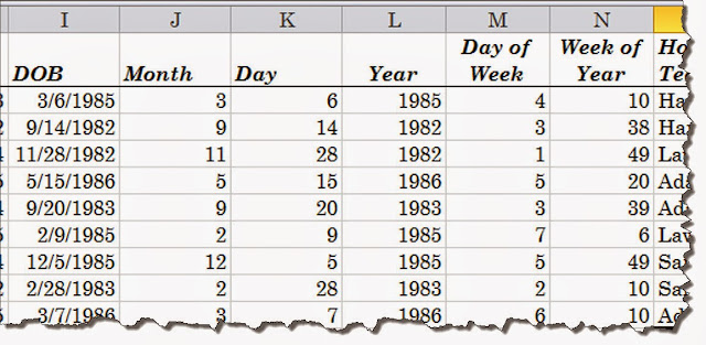
To change the format you need to select columns J through L. After they are selected go to the Home tab and in the Number group choose a General format. Now the results are displayed properly. All you have to do is select these three cells by dragging across them. Release your mouse button and double click the little fill handle in the lower right side of the selected cells. Presto! The cells fill down and you're ready to sort by any of these fields.

WEEKNUM Function
When doing an analysis of the information you have, it might be helpful to be able to group the information by week. If that is the case then you need to know what week number, from 1 to 52, the date represents. The WEEKNUM function will return that based on the date in your worksheet. Like the other date functions we're reviewed, the WEEKNUM function uses the one argument. Again you might want to insert a new column for this information. After you have done that, click in the first cell and insert the WEEKNUM function from the Formulas tab, Function Library, Date & Time group. Format the results if necessary and fill the formula down using the fill handle. Now you can analyze the information by weeks of the year.

You'll notice when you are in the Function Builder dialog box that there is an Return_Type field. This field is optional and is used to determine how the first week of the year is calculated. Leaving it blank assumes you are using System 1 as described below. Type a 2 in this field if you want to use System 2.

• System 1    The week containing January 1 is the first week of the year, and is numbered week 1.
• System 2    The week containing the first Thursday of the year is the first week of the year, and is numbered as week 1. This system is the methodology specified in ISO 8601, which is commonly known as the European week numbering system.

WEEKDAY Function
Suppose you wanted to see the production that occurred on a particular day of the week so that you could see productivity trends. You would need to know what day of the week a particular date represented. For that you would use the WEEKDAY function to parse that information out. Insert a new column for the weekday information. After you have done that, click in the first cell and insert the WEEKDAY function from the Formulas tab, Function Library, Date & Time group. Format the results if necessary and fill the formula down using the fill handle.By default Sunday is represented as 1, Monday as 2 and so forth. You can use the Return_Type option in the Function Builder dialog box to change the numbering sequence. Visit the Microsoft website if you need more information on changing the sequence for returning the weekday number.

I hope you can use these functions to further analyze information you have that includes dates.

My second book, Excel's Amazing Pivot Tables, should be out in a few months. Click the Subscribe button on the right so I can let you know when it's available for purchase.

Happy Computing!

Diane

Don't forget to click the Subscribe to 100 Computer Tips in 100 Days via email link on the right side of the screen so you get email alerts when Diane adds a new post.

Want more tech news or interesting links? You'll get plenty of both if you keep up with Diane McKeever, the writer of 100 Computer Tips in 100 Days, by subscribing to her Facebook posts or visiting her web page, www.dianemckeever.com . 

Recover Written Over Files

For Life's Uh-Oh Moments - Recover Written Over Files

I bet you've been there more than once in your life. You have a Microsoft Office document open (Word, Excel, PowerPoint, etc.) and you instinctively click the Save button...or better yet, use the Ctrl + s key to save...and then realize you meant to use the Save As feature rather than Save! Uh-oh, that original document has been written over and you can never recover it! But wait, there is hope!

Many years ago Microsoft realized that being able to recover previous versions of a document was a valuable feature so they incorporated it into all of their programs. You can access these previous versions by following these steps:

• Open the file that you want to restore to its previous version
• Click the File tab and click on Info
• On the right, select the version you want to open from the versions list
• Click the Restore button when the file opens

There, now won't you sleep more soundly tonight knowing that Microsoft has your back in this important way?

Like this tip? Want to get alerts when new tips are posted?  Click the Subscribe button on the right. 

Happy Computing!

Diane McKeever

Have you bought your copy of my book, "100 Amazing Computer Tips"? Click here to get one on Amazon.com. It's only $14.99 and it's packed with time saving tips. It makes a great gift any time of the year.

Amazing Tips - Recovering Unsaved Documents

Recovering Unsaved Documents!

Microsoft has your back on this!

How many times has this happened to you, you close a program quickly and in the "do you want to save changes" dialog box you reflexively click the "Don't Save" option...and then you realize that you didn't really mean to do that! This is usually followed by a burst of expletives as you mentally kick yourself for being so stupid. Well, Microsoft has your back on this. You can recover unsaved documents for up to four days from closing them!

To recover unsaved documents:

1. Open your program up again, if you closed it, and click on the File tab. 
2. Click on Recent and you will see in the lower right side of the screen those wonderful words...Recover Unsaved Documents (or Workbooks or Presentations, depending on program). 
3. Click the link and it will reveal that, unbeknownst to you, there is a folder labeled "Unsaved Files", created by your new best friends at Microsoft. Recent documents will be listed there for you to choose from. 
4. Click on a file and click Open
5. Now that your recovered document is open, don't forget to save your file!

Keep in mind the files in this folder are only saved for four days so don't dawdle, reopen the file quickly.

You might want to check the settings in your Office programs to see if this feature is turned on (it is by default) and adjust the AutoSave frequency. To do this:

1. Open the Office program (Word, Excel or PowerPoint)
2. From the File tab choose Options
3. On the left panel choose Save
4. Note the save documents settings and make sure that both Save AutoRecover information every XX minutes and Keep the last autosaved version if I close without saving have a check mark

The save button is still your best friend and the mantra I try to impress in my classes is to "Save Early and Often" which is still the best policy. But it's good to know you have Microsoft watching out for when you rashly close documents without saving!

Just a word about the AutoRecover setting of every 10 minutes, which is the default. If you want to minimize your exposure in case your document is unexpectedly closed, you might want to consider changing this to 5 minutes.

One more thing, you might have noticed the green arrow and box in the top picture of this post. Those are pointing to push pinned documents. For information on this great office feature see my post on this helpful topic.

Have you bought my book yet? If not, why not??  100 Amazing Computer Tips - Shortcuts, Tricks, and Advice to Help Everyone from Novice to Professional, is available NOW at Amazon.com and Barnes & Noble in both print ($14.99) and ebook ($7.99) formats. There's also a handy link on top right side of this window for your shopping convenience. If you've bought my book, THANK YOU! Please consider writing a review on Amazon.com.

Happy computing!

Diane

Don't forget to click the Subscribe to 100 Computer Tips in 100 Days via email link on the right side of the screen so you get email alerts when I add a new post.

Amazing Tips - The Art of Hovering

The Art of Hovering

Getting more from your software

I am frequently asked how I learn new software and keep current with new releases. The primary approach I use is to hover.

According to Merriam Webster, there are many uses for the word hover including:

• to float in the air without moving in any direction
• to stay very close to a person or place
• to stay near a specified point or level

When learning new software I am referring to the third use of hovering. I move slowly across any toolbars that are available, pausing at each item. As I do so a balloon label generally appears giving me some insight into the use of the tool. This is quite helpful because it is not uncommon that the icons defy deciphering and the balloon label is of limited help. At least at that point I can go to a browser and search for more information about the tool since I now know what it's called.

I think it's generational but, the graphic designers who come up with the size/shape/color of the tools often have different perspective than I do and different from the people I work with. In the early days of computers, the designers came up with the blue floppy disk to represent "Save". Twenty five years later I'm still pointing it out to people and explaining that it is the tool to use to save their work. The response I get is predictable. I hear everything from, "I thought it was a 50's TV set", to "What's a floppy disk." I used to carry a floppy in my bag to demonstrate the likeness to the save button but, without a machine to read them, my floppies didn't survive the last move.

One of my favorite discoveries that I found using the hover technique was to locate the "missing" dialog boxes I had become accustomed to using in Microsoft Office programs. When Microsoft did away with menus with the 2007 version of the office suite, I could no longer go to the Format menu to format text and paragraphs...not until I hovered and discovered the "Show dialog box" option on the ribbon. Now when I want to use advanced features in Word, features that the engineers didn't include on the ribbons, all I have to do is click the Show dialog box option.

Write a comment about a tool you learned about when you were hovering.

Have you bought my book yet? If not, why not??  100 Amazing Computer Tips - Shortcuts, Tricks, and Advice to Help Everyone from Novice to Professional, is available NOW at Amazon.com and Barnes & Noble in both print ($14.99) and ebook ($7.99) formats. There's also a handy link on top right side of this window for your shopping convenience. If you've bought my book, THANK YOU! Please consider writing a review on Amazon.com.

Happy computing!

Diane

Don't forget to click the Subscribe to 100 Computer Tips in 100 Days via email link on the right side of the screen so you get email alerts when I add a new post.

Amazing Tips book now available

Amazing Tips, the book, has been released!

I am pleased and excited to announce that my book, 100 Amazing Computer Tips, is finally available from Amazon in both print and ebook formats.

The book is based on the top 100 tips in this blog, which were reorganized and expanded. In addition I included printable tip cards for many of the popular software programs.

100 Amazing Computer Tips is the first in a series of Amazing Tips books that will be developed on a wide variety of subjects. I will be writing many of the computer based books but am looking for writers to author books on other topics. The Amazing Tips books could become the new Dummies series...but for smart sophisticated people like you! If you, or anyone you know, would like to be considered for the Amazing Tips series, please contact me.

You can go to Amazon.com NOW and make your choice there between the print and ebook formats. The print version is 14.99 and the downloadable ebook version is 7.99. If you've already bought a book, thank you. I hope you would consider reviewing it on Amazon for me. Your feedback is important.

Happy Computing!

Diane

Don't forget to click the Subscribe to 100 Computer Tips in 100 Days via email link on the right side of the screen so you get email alerts when Diane adds a new post.

Want more tech news or interesting links? You'll get plenty of both if you keep up with Diane McKeever, the author of 100 Computer Tips in 100 Days, by subscribing to her Facebook posts or visiting her web page, www.dianemckeever.com .