Named Cells and Ranger in Excel

Great Computer Tips

Named Cells and Ranges in Excel

Naming cells

Cells already have names such as A1, B27, etc. but you can also give them names to make it easier to reference that specific cell, making the cell address (name) an absolute reference rather than the default relative address. In the image below, you might want to name cells A1 through D10 but since you might be expanding your product list we'll give columns A through D a name.

• Start by selecting the single cell, range of cells, or columns you want to name.
• Click in the name box (the name box is in the upper left side of your screen, just above the first column, see image to the right) and type a name for your cells.
• Press the Enter/Return key. This step is very important.

If we called this area of our worksheet "table" we would be able to use the word "table" in our formula and Excel would know that we were referencing these cells on this worksheet. 

Note: When naming cells you need to remember that you can not use spaces and the name can not begin with a number. Also remember, the name must be unique in the workbook because the name refers to a location in a specific worksheet in the workbook. 

Using Names in Formulas

Once you have named a cell or range of cells, you can insert that name into your formula. The formula becomes easier to decipher and doesn't require adding $'s to the cell address to make it a fixed location. The formula could be =SUM(sales) rather than =SUM(A3:G27).

Viewing the Names in a Workbook

You can easily view all the names in the workbook by clicking the down arrow on the right side of the Name Box. The list is always viewed in alphabetical order.

Happy Computing!

Diane

Don't forget to click the Subscribe to 100 Computer Tips in 100 Days via email link on the right side of the screen so you get email alerts when Diane adds a new post.

Want more tech news or interesting links? You'll get plenty of both if you keep up with Diane McKeever, the writer of 100 Computer Tips in 100 Days, by subscribing to her Facebook posts or visiting her web page, www.dianemckeever.com

Creating Mosaic Pictures

100 Computer Tips in 100 Days

Creating Mosaic Pictures

The original picture

I’m sure you've seen pictures that are made up of hundreds of little pictures pieced together into a mosaic. I often wondered how they could do something like that and recently discovered that many websites will make one of these. Of course, you supply both the primary picture and the individual pictures that will make up the mosaic but it’s not really that much work, and I’m here to help you!

The first thing you need is a clear, crisp, high-quality image that will be made into the mosaic. This could be a picture of an individual or a landscape. In my example, I have used one of the sample pictures that came with your computer.

Here's a sample of the picture files I used for my mosaic.

Next, I did a Google image search for blue, yellow, and green images. Remember that when you do image searches you can click on the Search Tools button along the top of the screen and you can search for images based on many attributes, including color. Look for pictures that are primarily made up of the color you are looking for. Too much white around the edge won’t translate well.

Use the Google Search tools to identify pictures made up of specific
colors. You want a good distribution of the primary colors used in your
image.

As you find pictures you can right-click on them and choose Save Image  (See Tip #46). Collect the pictures into a new folder so that you can easily find them later. Depending on how large the area is for a particular color you should probably find 35 or 50 images of each color.  Remember that individual pictures may be used more than once in the final mosaic.

The final results!

I used the Easy Moza website (www.easymoza.com) and it was very easy. I chose this site because you didn't have to download the program. I'm not keen on downloading unnecessary software. There is no cost to create a mosaic and download a low-resolution file of the finished product. If you need a higher resolution you can purchase it. Your finished product can be printed out on your local printer or emailed to Staples/Costco/CVS for printing and framed for a nice gift.

Happy Computing!



Diane

Don't forget to click the Subscribe to 100 Computer Tips in 100 Days via email link on the right side of the screen so you get email alerts when Diane adds a new post.

Want more tech news or interesting links? You'll get plenty of both if you keep up with Diane McKeever, the writer of 100 Computer Tips in 100 Days, by subscribing to her Facebook posts or visiting her web page, www.dianemckeever.com . 

Tip #117 - Tis The Season To Mail Merge

100 (or more) Computer Tips in 100 (or more) Days

'Tis the Season to Mail Merge 

I was reminded of this tip when my phone started ringing and my inbox filled up with requests for my Mail Merge tip card. Everyone is using Mail Merge this month to get the labels printed to mail the Christmas - Hanukkah - New Year's cards and newsletters. The process is not that difficult but there are, of course, some pitfalls that you can fall into. Let's start with a description of a mail merge.

Mail Merge

Mail Merge is the process of taking a single form letter, combining it with a list of names and other information, and then merging both to create several customized documents. The results of a mail merge are generally personalized letters and labels. This post will assume you want to create labels. If you need something else I think you will be able to do that after following these instructions.

The file that contains the names and other information is the data source. The file that contains the form letter/label template is the main document.

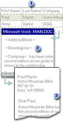
Documents in a Mail Merge

1. Data sources with recipient information, such as names and addresses
2. Main document with merge fields that are placeholders for recipient information
3. Resulting merged document

Task Pane

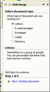
This feature of Word is executed by following the directions in the Task Pane. The Task Pane appears on the right side of your screen when the Mail Merge task is selected.

Getting Started

Create a data file. I recommend using Excel for the data file. Even if you've never used Excel before, it's easy to put names and addresses in the columns and rows of an Excel document. Look at some Excel tips, such as auto-resizing columns for assistance. Make sure that row 1 in the Excel document has the column labels such as "first name" and "last name". You will use these in step 4 of the mail merge to identify what information goes where. 

If your information is in Outlook I would recommend that you export the names to an Excel file. You generally need to do a lot of cleaning up of the information before you do your merge and it's really easy to do that in Excel.

Getting Started

To make the mail merge process easier we will use the Mail Merge Task Pane. The Task Pane will walk you through the six steps necessary to complete the merge. While it is possible to do a mail merge without bringing up the task pane I don't recommend it.

In Word 2007 or newer

Click the Mailings Tab —> Click the “Start Mail Merge” option —> Step by Step Mail Merge Wizard. 

In either version, the task pane will appear on the right side of the screen. Apple users will see a floating pane that will have the numbers one through six. As we walk through the steps you will go to each section.

Steps in the Mail Merge Task Pane

Step 1 – Select document type: letters, email messages, envelopes, labels, or directory. In our example, we will be making mailing labels.

• Letters – personalized letters
• Email messages – Outlook messages
• Envelopes – mailing envelopes
• Labels – any type of Avery-type labels
• Directory – a catalog of information such as a telephone directory

·

Step 2 – Click “Next: Starting document” – set up the document by choosing label type or document type. 

Because the Word document on your screen is probably not a label document, click Change Document Layout and click the Label Options link.

In the Label Options dialog box, in the Label Vendors section choose "Avery US Letter". When you do this you will see all of the hundreds of Avery labels listed. Look at the box of labels you bought and check the number you should be looking for. Avery 5160 is the most popular size resulting in a sheet of 30 labels per page in three columns. When you return to your document after choosing the label template you should see your document divided into cells. NOTE: If you can not see the cell gridlines click on the Table tab, Format, and choose View Gridlines.

·

Step 3 – Select recipients — this step is asking you to identify the file where the names are coming from. 

Click Browse and find your file. If you are choosing an Excel document a second window will appear after you click open. This second window confirms the name of the sheet in Excel. Most people will use Sheet1.

A third window will appear with the Excel information. Use the checkboxes to exclude individuals from the mail merge. The data can also be sorted by clicking on the column headings. Click OK.

Step 4 – Arrange document – Insert the fields into the main document

• In Word for Apple, drag the fields from the Mail Merge Palette on to the document.

• In Word 2007 or newer click the Mailings Tab — Insert Merge Fields option - make sure you click on the WORDS Insert Merge Fields and not the button itself. If you click on the button a dialog box will appear. If it does just cancel and click the words. Insert each field in the order you want them on the label. Insert spaces and returns between fields where necessary. Don't worry if the text wraps, it probably will be OK when the merge is completed.

• If creating labels, Click the Update All Labels button to add the same fields to all labels. This is also an opportunity for you to add graphics, change fonts, etc.

Step 5 – Preview your labels

• If any adjustments are needed, click the Previous hyperlink to return to step 4 and make adjustments

Step 6 – Complete the merge

• Print – will print the list (labels or document)
• Edit individual labels (letter) – creates a file you can save and edit and use again. This is the option that I strongly recommend. 

à Choose All records, (recommended) a Current record, or identify a range of records, click OK

A new document appears with all of the names merged. This is the document you will print. Saving it is a good idea. Scroll through this merged document making any changes necessary to the individual labels.

Hope this helps.

Please share this tip with your friends, they'll thank you for it.

Happy Computing!

Diane

Don't forget to click the Subscribe to 100 Computer Tips in 100 Days via email link on the right side of the screen so you get email alerts when Diane adds a new post.

Want more tech news or interesting links? You'll get plenty of both if you keep up with Diane McKeever, the writer of 100 Computer Tips in 100 Days, by subscribing to her Facebook posts or visiting her web page, www.dianemckeever.com . 

Excel - Converting Zip Codes to City and State

 100 Computer Tips in 100 Days

Excel - Converting Zip Codes to City and State


In my new position, I offer free webinars to people who want to improve their chances of business success. These folks sign up with their name, email, and zip code. I was curious about their location and was amazed that Excel could convert the zip codes into city and state locations. BTW, I believe this feature is only available in the 365 version of Excel.

To do this you need to start by converting the zip code column to text. 

1. Select the zip code column by clicking on the letter of the column
   
2. From the Home Tab, Number Group, choose Text

Select all the zip codes in the list 

1. Click the first zip code and use the Ctrl + down arrow key
2. From the Data Tab, Data Type Group, choose Geography

You will see a new icon to the left of the zip code entries

Select the first zip code in your list. You will see a new icon on the right, the Insert Data icon. Click it and choose "City". 

The City and State will be inserted into the cell to the right of the zip code. Use the fill handle to fill this code down the rest of your list. You may get some wonky entries if incorrect data is entered. 

I hope you enjoyed this tip. Please share the link to your friends.

Diane

Diane McKeever, CPP

Certified Patient Person

Don't forget to click the Subscribe to 100 Computer Tips in 100 Days via email link on the right side of the screen so you get email alerts when Diane adds a new post.

Capturing a Portion of a PDF for Printing

Amazing Tips - Capturing a portion of a PDF for printing 

Only want to print a section or area of a PDF page? Here's how

A little background on PDF files:

It became apparent years ago that there needed to be a file type that would allow people to view documents that were created in unique programs, programs that not many people used, without the viewer actually having the software on their computer. This was a problem that graphic designers and architects and the like were having when they wanted to share their creations with clients who didn't own the expensive software. Their clients couldn't be expected to purchase programs that cost hundreds and thousands of dollars just to view the designs so Adobe (and others) developed PDF (Portable Data Format) files.

Soon all computers came with the free Adobe Acrobat Reader so that you could view all kinds of files but to create a PDF you still needed the full Adobe Acrobat program, which wasn't free. Of course, third-party providers sprang up to fill the void. Adobe worked then with software companies to enable the creation of PDF files from just about any program, which is the case now.

Why are PDF files so important?

The main reason they became so important was for file sharing but other reasons to use PDFs soon became apparent. If you were sending a contract that was written in Microsoft Word but you wanted to make sure no changes were made to it, you could convert the document to a PDF. Another popular reason to create a PDF is that the file size is much smaller than the file in the native program would be.

Printing a section of a document

The print dialog box has always given you the opportunity to print specific pages. I often scroll down the document, making note of the pages I would like to print so that I don't waste paper. Then when I click on the "print" command I fill in the page numbers as they are in the graphic below. Specific pages are listed separated with a comma and ranges of pages use a dash between the page numbers. Of course, this is not just in a PDF program, this works in virtually all programs.

Printing a portion of a PDF page

OK, so this was the initial problem, you wanted to print just a portion or section of a PDF page. Adobe has given you a tool to do just that. 

1. Open any PDF document and scroll to the area you would like to print
2. From the Edit menu choose "Take a Snapshot"
3. Now drag in your document to select the specific area you would like to print
4. Click the print icon OR choose print from the file menu OR use the keyboard shortcut Ctrl + p
5. In the print dialog box you'll notice you have an option to print "Selected graphic", which is your highlighted section of the document and to Scale the selected graphic. I love using the "Fit" command because it will increase/reduce the graphic as necessary to fit on a sheet of paper. You can plan with the other commands in the Scaling section to see which gets the best results for your purpose.

This is pretty dandy stuff but it only works in a PDF document. For other documents, you might want to use the Snipping tool which was described in a previous blog post. Click the link to see the details of that great tool.

Have you bought my book yet? If not, why not??  100 Amazing Computer Tips - Shortcuts, Tricks, and Advice to Help Everyone from Novice to Professional, is available NOW at Amazon.com in both print ($14.99) and ebook ($7.99) formats. 

If you've bought my book, THANK YOU! Please consider writing a review on Amazon.com.

Happy computing!

Diane

Tip 105 - Alt Code Reference Sheet

100 Amazing Computer Tips

Tip #105 - Alt Code Reference Sheet

Have you ever wondered how people inserted special characters such as smiley faces, hearts, arrows, etc. into their emails, Tweets, Facebook posts, or worksheets? They probably used Alt codes to accomplish it. This sheet has been downloaded over 40 thousand times!

Alt codes have been around for decades and were used by early programmers. I have compiled a list below for your use. For best results, you should save the picture by clicking on it with the right mouse button and choosing "Save Image As" or "Save Picture As" and saving it on your desktop. You can then double-click the image on your desktop and print from there. 

After this was posted my Apple friends were very sad that they couldn't do this fun stuff with the Alt key. Here's a special character reference sheet for you. Hope this helps my Apple friends.

If you like this tip, go to the index  to see if there's more posts to make you a more effective computer user.

Happy Computing!

Diane 

Have you bought my book yet? If not, why not??  100 Amazing Computer Tips - Shortcuts, Tricks, and Advice to Help Everyone from Novice to Professional, is available NOW at Amazon.com and Barnes & Noble in both print ($14.99) and ebook ($7.99) formats. There's also a handy link on top right side of this window for your shopping convenience. If you've bought my book, THANK YOU! Please consider writing a review on Amazon.com.

Happy computing!

Diane

Don't forget to click the Subscribe to 100 Computer Tips in 100 Days via email link on the right side of the screen so you get email alerts when I add a new post.

Excel's Amazing VLOOKUP Function

Great Computer Tips

Excel's Amazing LOOKUP Functions

The LOOKUP functions in Excel are so powerful but so confusing to many. Part of the problem is the terms that Excel uses when defining the arguments. Let's see if I can make things clear for you.

LOOKUP functions copy information from a table based on data in specified cells. You see LOOKUP functions in use all of the time. The bar code scanner in stores uses a form of lookup. The scanner identifies the UPC number and returns the name of the item and the price from a list stored on the server. The UPC is the trigger or the number being looked up and the price is in one column and the name of the item is stored in another column. I can hear you saying that you're not selling products and don't use UPC numbers. Another example of a lookup is auto-entering customer information using a customer number.

This VLOOKUP uses an Item # that is common to the worksheet and the Lookup Table to automatically import information.

For many years I was in charge of scoring sailboat races and we used an Excel worksheet to accomplish this. When a boat came out to race we entered the sail number and the spreadsheet looked up information from another sheet that had hundreds of sailboats listed. The sail number would trigger the lookup and the name of the boat would be automatically entered as well as the name of the skipper and the handicap.

In a recent tip for parsing date information into individual segments, I suggested the use of the WEEKDAY function to determine the day of the week that a particular day falls on. The result of this formula is a number from 1 to 7. If you wanted to convert those numbers to day names (Sun, Mon, etc.) then you would consider using a lookup to accomplish this task.

So now that you have some ideas about how you would use a lookup let's get started.

Setting up the Lookup table
The data in the table needs to be set up so that the lookup number (the information you are looking for such as the UPC code or model number) is in the leftmost column and is sorted in ascending order (from smallest to largest). To make it easier to identify the location of the table the next step would be to name the table area.

Naming cells
Cells already have names such as A1, B27, etc. but you can also give them names to make it easier to reference that specific cell, making the cell address (name) an absolute reference rather than the default relative address. In the image above you would want to name cells A1 through D10 but because you might be adding to your product list we'll give columns A through D a name.

• Start by selecting the cells or columns you want to name.
• Click in the name box (the name box is in the upper left side of your screen, just above the first column, see image to the right) and type a name for your cells.
• Press the Enter/Return key. This step is very important.

If we called this area of our worksheet "table" we would be able to use the word table in our formula and Excel would know that we were referencing these cells on this worksheet. Note: When naming cells you need to remember that you can not use spaces and the name can not begin with a number.

Inserting the LOOKUP Function

Now that we've got the data range named lets look at how to construct the VLOOKUP function. Look at the image below, we will be inserting information in the worksheet on the left by looking it up in the sheet on the right.

In the example we will create a function to look up the description of an item based on the Item #. In the first cell in the description field, choose VLOOKUP from the Formulas tab, Function Library group, Lookup & Reference option. We are using a VLOOKUP rather than a HLOOKUP because the data we're looking up from in the worksheet on the right  is structured in a vertical format.

• In the function builder dialog box put in the cell address of the trigger cell. In this case it is cell B20, the cell that will contain the item #. 
• In the second field type the name that you gave your look up information. I named mine "table" so that's what I typed in here. 
• In the third box identify the column in the worksheet on the right that has the information you want returned. The Code (Item #)  is column 1, Description is column 2, Price is column 3 and Color is column 4. In this case we would type a 2. 
• If it is important, as it is in this case, that if there is no exact match to the Item # to return an error code, then in the fourth box enter the word "False" in the fourth field. When finished click OK.

That's it! Change the Item # and see if the results change. If it all looks good create the VLOOKUP function in the other cells.

You may notice that I refined the formula a little so that the formula didn't return an error message when the Item # cell was blank. You can see how this formula is structured by looking on the formula bar in the picture above.

Because this is a little complicated, I created a video and posted it on YouTube. Click here to see the video.

Happy Computing!

Diane

Don't forget to click the Subscribe to 100 Computer Tips in 100 Days via email link on the right side of the screen so you get email alerts when Diane adds a new post.

Want more tech news or interesting links? You'll get plenty of both if you keep up with Diane McKeever, the writer of 100 Computer Tips in 100 Days, by subscribing to her Facebook posts or visiting her web page, www.dianemckeever.com . 

Creating a video from a powerpoint presentation

100 Amazing Computer Tips

Creating a Video from a PowerPoint Presentation

Creating videos to support your social media efforts has never been easier. With a budget of zero you can create an awesome PowerPoint presentation, complete with audio, transitions, and animations, and turn it into a video. Turns out it couldn't be easier!

IMPORTANT: This feature was added to the 2010 version but if you're still using something earlier than that, you you should upgrade your software.

Create your presentation

Of course, step 1 is to create your PowerPoint presentation. For some of you, this might be the most difficult part. I can't give you a step-by-step of that process here, but look around the internet for some videos on creating a presentation, adding transitions between slides and animation to have text appear, dance around, and possibly disappear, being replaced with other words. All of this might sound hard but it's really not. If you were closer you could stop by and I'd show you.

You can also add narration and timings to your presentation. If you're adding narration I would strongly suggest you write a script. I've heard too many "off the cuff" narrations that sounded really dumb! The best way to add timings is to go to the Slide Show tab and use the Rehearse Timings option. This will allow you to set the advance on the slides to something appropriate for each slide. If you do not set timings the default advance is 5 seconds. I set my timings in the Slide Sorter view in PowerPoint (View tab, Slide Sorter View). Once in the Slide Sorter view, I clicked the Transition tab and in the Timing group, I entered 00:02.00 in the timings box and clicked Apply to All. I then selected individual slides that I wanted to remain on longer and adjusted the timing for those.

I inserted a soundtrack on slide #1 and formatted it (Audio Tools, Playback tab) so that audio would "Play across slides". Also, make sure the checkbox for Hide During Show is selected so the icon will not be visible. Depending on the length of the audio file you might also want to check the "Loop until Stopped" option.

BTW, I found my audio online by doing a search for "40-second instrumentals free" and found a dandy one right away.

Before you save the audio you should optimize the audio file. To do this go to the File tab, Info, Compress Media. This will embed the media and make the file a reasonable size.

Save your presentation

You'll want to save your presentation as you are creating it of course. This baby isn't going to be created in one sitting...I guarantee that! Once it's saved as a PowerPoint document, follow the directions below.

1. On the File menu, click Save & Send.
2. Under Save & Send, click Create a video.
3. To display all video quality and size options, under Create a video, click the Computer & HD Displays down arrow.

• To create a video with very high quality, yet a large file size, click Computer & HD Displays.
• To create a video with moderate file size and medium quality, click Internet & DVD.
• To create a video with the smallest file size, yet low quality, click Portable Devices.

 TIP   You'll want to test these out to see which option meets your needs. In the video below I used the first option for a very high-quality video.

The saving process might take a few minutes so I walked away from my computer. When I came back there it was my finished video. I think it looks pretty good, don't you? This whole process probably took just about an hour. Now I'm going to upload the video to my website and even to my YouTube channel.

My book, 100 Amazing Computer Tips - Shortcuts, Tricks, and Advice to Help Everyone from Novice to Professional, is available NOW at Amazon.com and Barnes & Noble in both print ($14.99) and ebook ($7.99) formats. There's also a handy link on the top right side of this window for your shopping convenience.

Happy computing!

Diane

Don't forget to click the Subscribe to 100 Computer Tips in 100 Days via the email link on the right side of the screen so you get email alerts when Diane adds a new post.

Tip #31 - Generating Random Text

100 Amazing Computer Tips

Tip #31 - Generating Random Text

OK, I can hear you asking yourself, “Why would I want to generate random text?” Just bear with me.  There are many occasions when I need to do this and it’s very cool so I’m sharing it with you.

The programmers at Microsoft often need to generate random text to test software so they built in a secret macro that will produce a specific number of sentences and paragraphs made up of real words, not computer Latin words. Try this out in your Microsoft Word program.

Open a document in Word and type the following then press the enter key (return in Apple world):

=rand(5,7) d

Presto, the code you typed changed to five paragraphs each containing seven sentences. Keep in mind that the five and seven could be any two numbers depending on how much random text you need. So the next time you need to demonstrate something in Word to a colleague and you need some text to use, remember the code. It’s pretty easy if you keep in mind that rand stands for random.

If you would rather have Latin words rather than distracting English words, you can do that too. Type =lorem(5,7) in your document and then press the enter (return) key and it’s replaced with Latin text. Remember that five and seven can be any numbers you choose.

You can use this tip when you’re trying to show friends or coworkers some special word features and need to have some text to practice on. 

Happy Computing!

Diane

Buy my book at Amazon.com. It's only $14.99 and it's packed with 100 Amazing Computer Tips! They're nicely organized and really easy to follow.

Don't forget to click the Subscribe to 100 Computer Tips in 100 Days via email link on the right side of the screen so you get email alerts when Diane adds a new post.

Want more tech news or interesting links? You'll get plenty of both if you keep up with Diane McKeever, the author of 100 Computer Tips in 100 Days, by subscribing to her Facebook posts or visiting her web page, www.dianemckeever.com . 

Fine Tuning Your PowerPoint Skills

My PowerPoint Pet Peeves!

I recently attended a virtual meeting on Zoom...of course...and the presenter did a great job of explaining his subject matter but I was so distracted by a few issues with his PowerPoint document that I was having trouble concentrating! Let's talk about some of my PowerPoint pet peeves.

• Bullet items written as complete sentences
• Periods in bullet lists
• Revealing the complete bullet list all at once
• Numbers not correctly aligned

Bullet List "Rules"

The core of most presentations are bullet lists. Here are a few "rules" you should keep in mind if you are creating a presentation using them. 

• Do not write the bullet as a complete sentence. It is your job as the presenter to speak in sentences but your audience should not see your complete thought written out. They will have difficulty remembering a full sentence so write your bullet as thoughts or phrases.
• If you follow the advice of the above bullet, you should not be using punctuation in your lists. If the bullet is not a complete sentence, it does not need a period at the end of it! Feel free to use exclamation points or question marks but no periods.
• Use the animation feature in PowerPoint to reveal the bullets one at a time. Doing this will direct your audience's attention to the current bullet and not to the upcoming bullet points. It is not necessary to use some of the more distracting animations (grow & turn, swivel, and bounce) designed to spice up a 5th graders show, a simple "appear" is a good choice. 
• Keep the number of bullets on a slide to five or six. If you have more than that you should consider splitting the information into multiple slides.

Aligning Numbers

Sooner or later a presentation you are making will contain numbers. If the numbers all have the same number of digits you are in luck. You can simply use the tab key to move to the right and type your numbers. For the rest of you, you may resort to using the space bar to move to the right in hopes that the result will get the numbers to appear to be aligned on the right side...this is a pretty hit and miss approach. The best approach is to set a right align tab and use the Tab key to get those numbers straight. Here's how you do that.

1. Click in the text block where you will be inserting the numbers
2. If you see a ruler across the top of your screen you're golden. If you do NOT see a ruler, click the View Tab, Show Group, Ruler.
   
   
   
3. On the far left side of the ruler, you will see the Tab Box. This is where you select the alignment type you need to place on the ruler. Your options are left, center, right, and decimal. As you click this box the image changes to reveal the four types. Click until the right alignment tab is displayed in the box, it looks like a reverse "L". (See picture below)
   
   
   
   
   
4. Once the right tab is displayed in the Tab Box, move your mouse to the ruler and click where you estimate the right side of the number list should be placed. The right alignment icon will appear on the rules. Now, as you type your entries, use the Tab key to jettison to the set tab. Type your number and it will build to the left and align on the right side!
   

   

   
   
   
5. If you determine that the tab on the ruler should be moved left or right, select the list and drag the ruler tab left or right. The numbers will move accordingly. 

Now you can concentrate on your content and getting your point across in your presentation and not fret about the little things like bullets and number alignment!

Happy Computing!

Diane McKeever

---------------------------------------------------------------------

Have you bought my book yet? If not, why not??  100 Amazing Computer Tips - Shortcuts, Tricks, and Advice to Help Everyone from Novice to Professional, is available NOW at Amazon.com in both print ($14.99) and ebook ($7.99) formats. 

If you've bought my book, THANK YOU! Please consider writing a review on Amazon.com.

Top Ten Posts for the Last Week

100 (or more) Computer Tips in 100 (or more) Days

Top Ten Posts for the Last Week







Want to know what posts your friends are looking at? Here's a list of the top ten posts for the past week. Have you checked all of these out?

• Tip #1 - Basic Mouse Actions 

• Tip #46 - Excel AutoFit Column Width 

• Tip #55 - Extra Help for Microsoft Office 

• Index by Category 

• Tip #106 - Facebook Graph Search Feature 

• Tip #99 - Excel Finding Duplicate Records 

• Tip #65 - Excel Formula Auditing 

• Tip #93 - Excel Scenario Manager 

• Tip #107 - Excel Pivot Tables 

• Top 10 Excel Tips

It's amazing to me to see that the top tip is about basic mouse actions. It's also clear that Excel is a very popular topic. I will be posting additional Excel tips in the next week, along with some video clips of the techniques. 

Happy computing!

Diane

Don't forget to click the Subscribe to 100 Computer Tips in 100 Days via email link on the right side of the screen so you get email alerts when Diane adds a new post.

Want more tech news or interesting links? You'll get plenty of both if you keep up with Diane McKeever, the writer of 100 Computer Tips in 100 Days, by subscribing to her Facebook posts or visiting her web page, www.dianemckeever.com . 

Tip #104 - Push Pin Office Documents

100 (or more) Computer Tips in 100 (or more) Days

Tip #104 - Push Pinning Documents

This is the one tip I use all the time to help you re-open frequently used documents.

Microsoft Office has always kept track of recently opened documents and you could see a list of the four most recent documents at the bottom of the File menu. In 2007 Microsoft expanded this list to display the last eighteen documents. At the same time, they included the option to pin a document to the list so that it would never roll-off, making it a cinch to open frequently used documents again. 

When you visit the File tab in any MS Office program (or the Office Button in 2007), you'll notice that when you click on Recent on the left panel two columns appear to the right. The left column contains recently used documents, the right column displays recently visited folders. Both of the columns have push pins available to the right of each entry. Click the pin once to "pin" the document/folder to the menu. 

This feature is particularly outstanding for those of you who are in a network environment where you have to do many clicks to navigate to network drives. Those drives are available now with one click.

Happy computing!

www.dianemckeever.com